Analyzing Camera Trap Pictures with AI
Using SpeciesNet (Google AI) to sort through hundreds of thousands of wildlife pictures from motion detection cameras (camera traps).
Skip to the good part:
Preview page created using Megadetector dev-tools on a subset of predictions.
Urban Rivers - CamTrap AI Observations
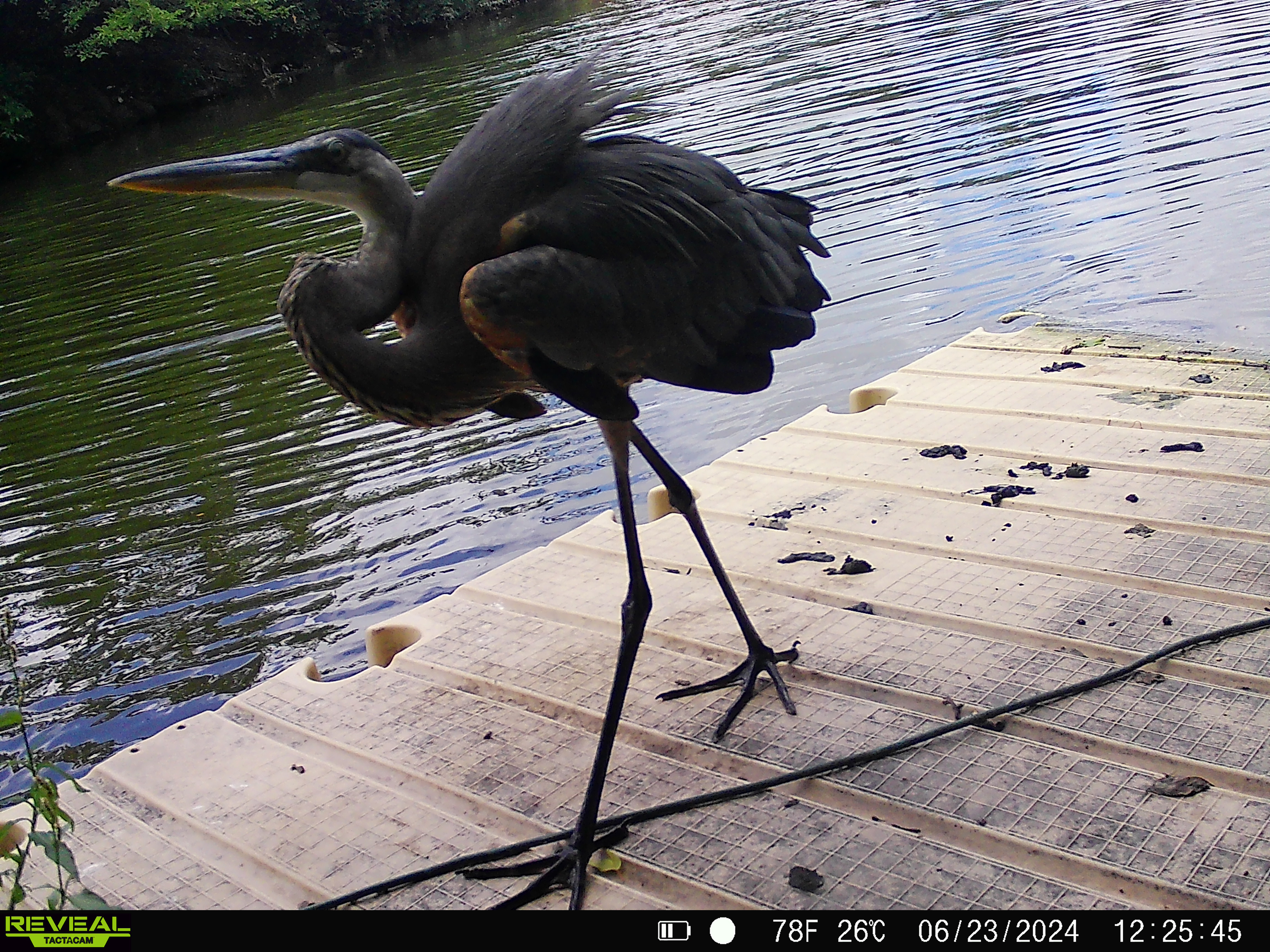
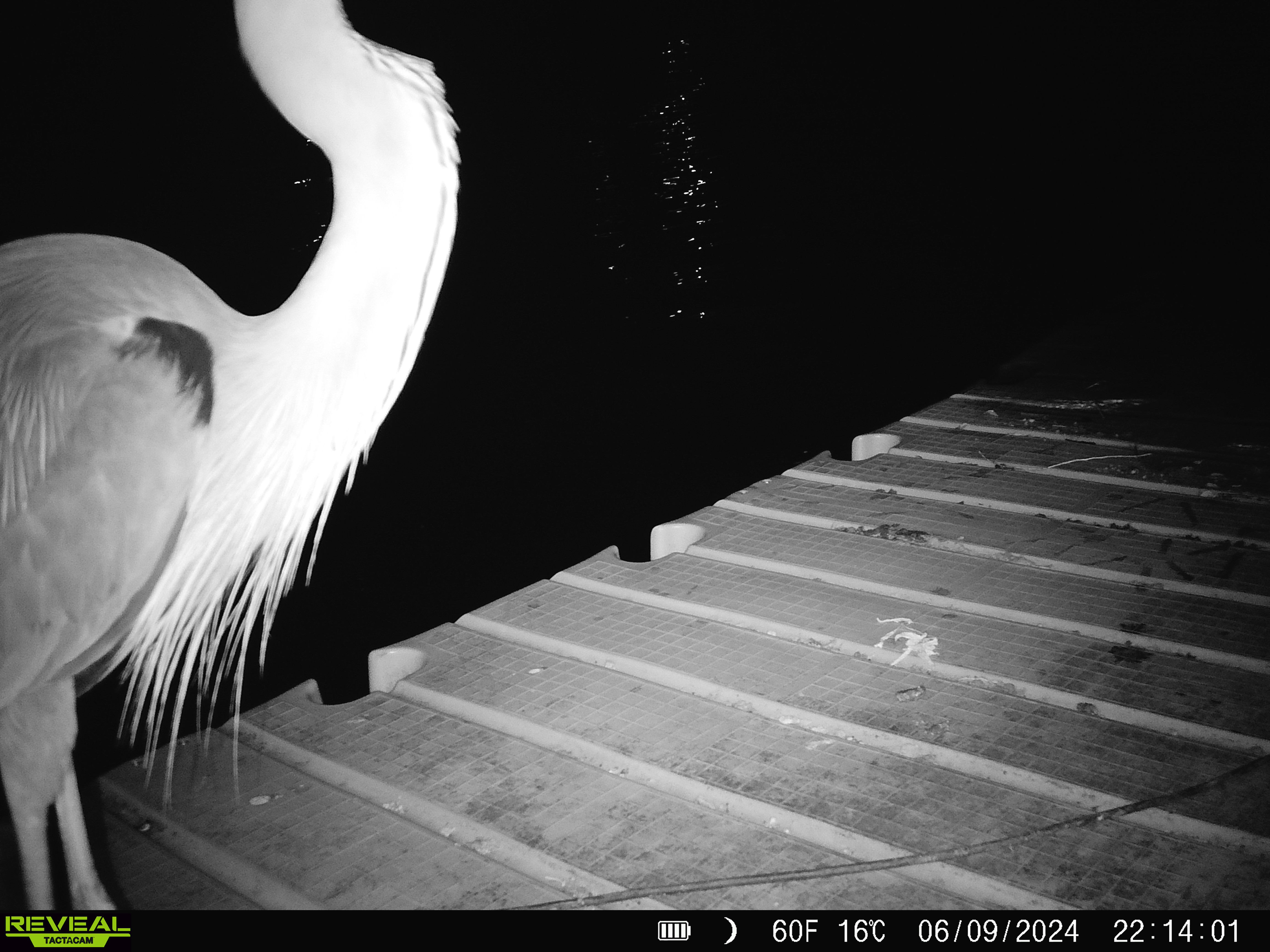
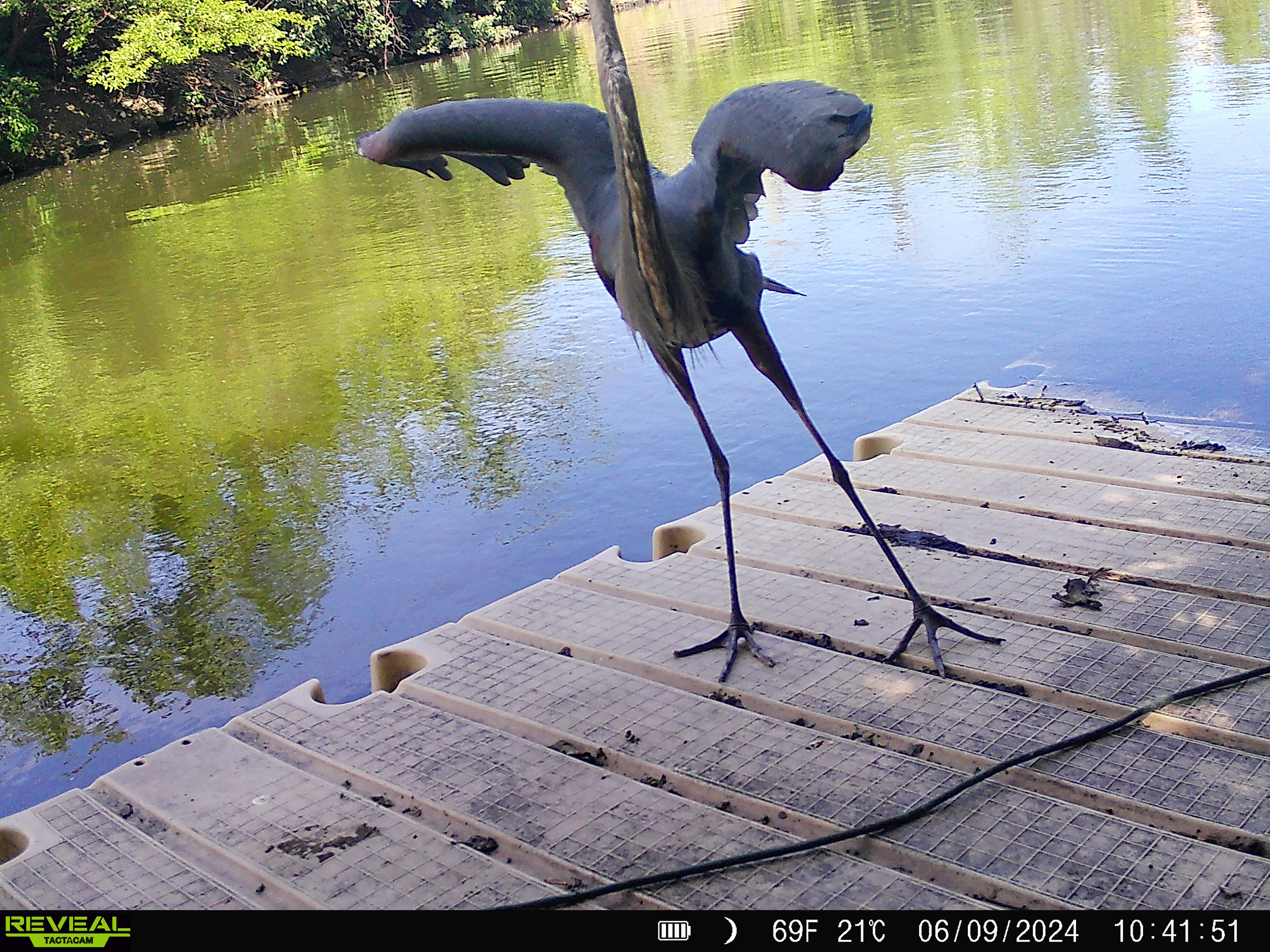
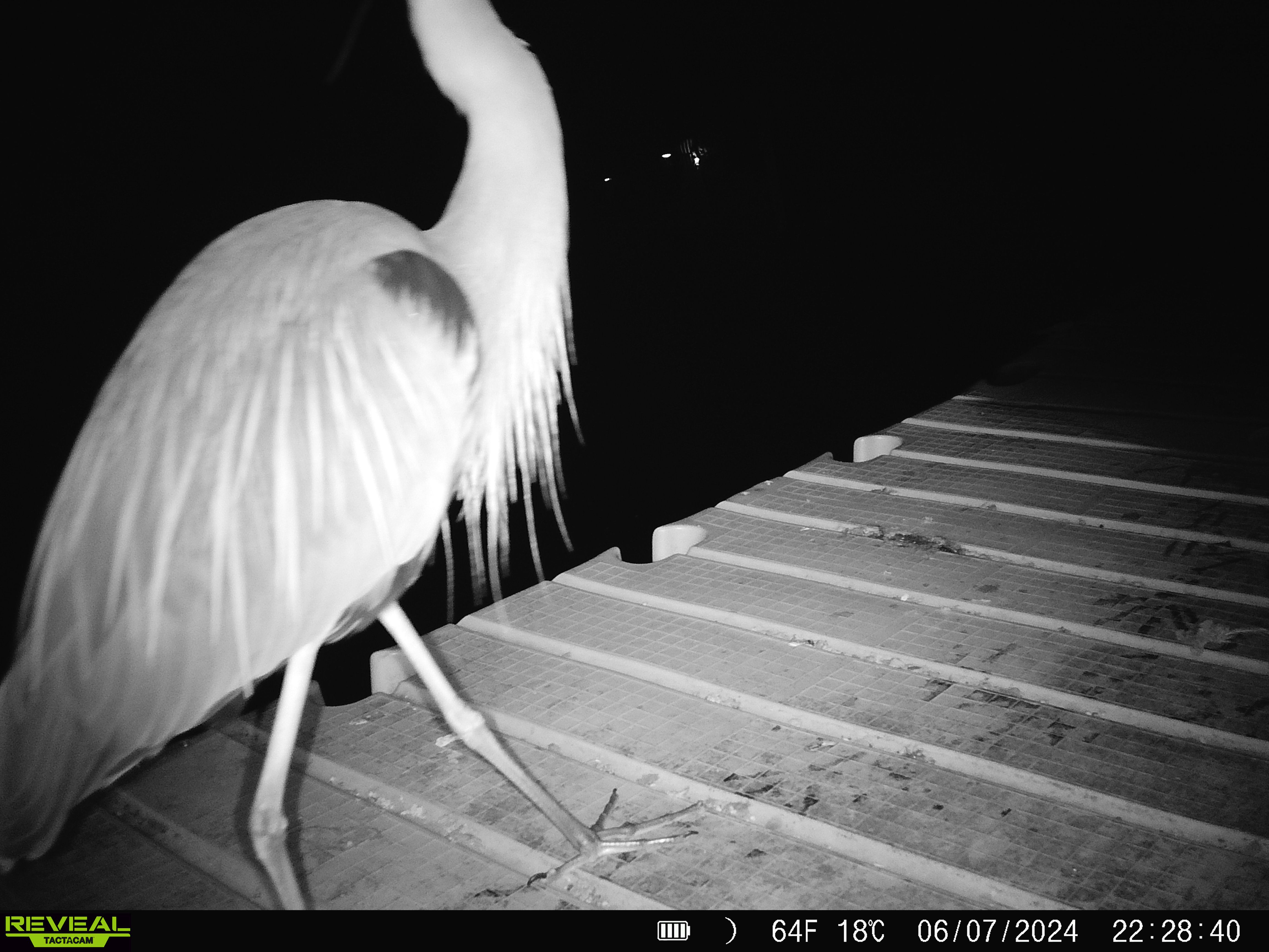
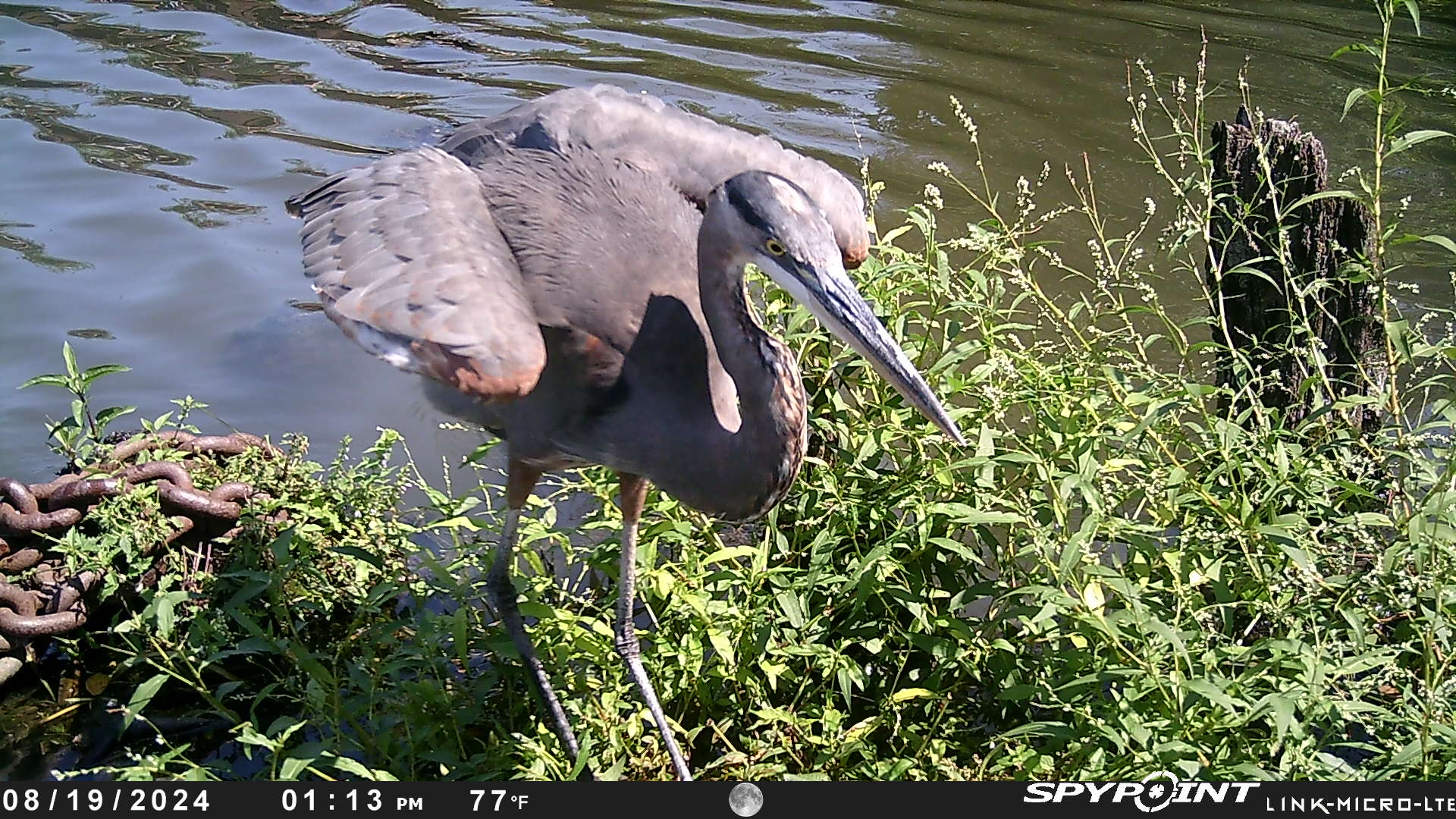
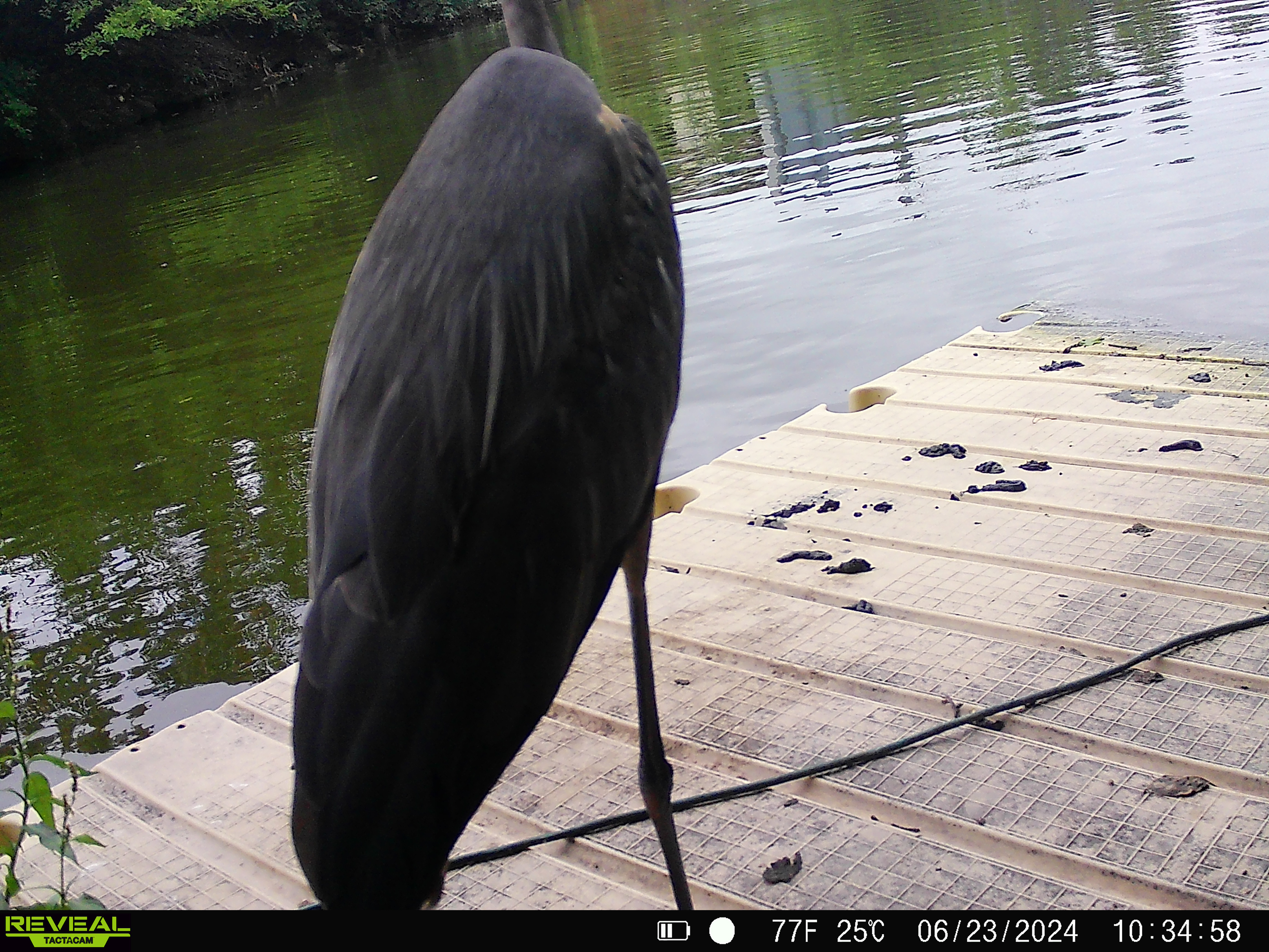
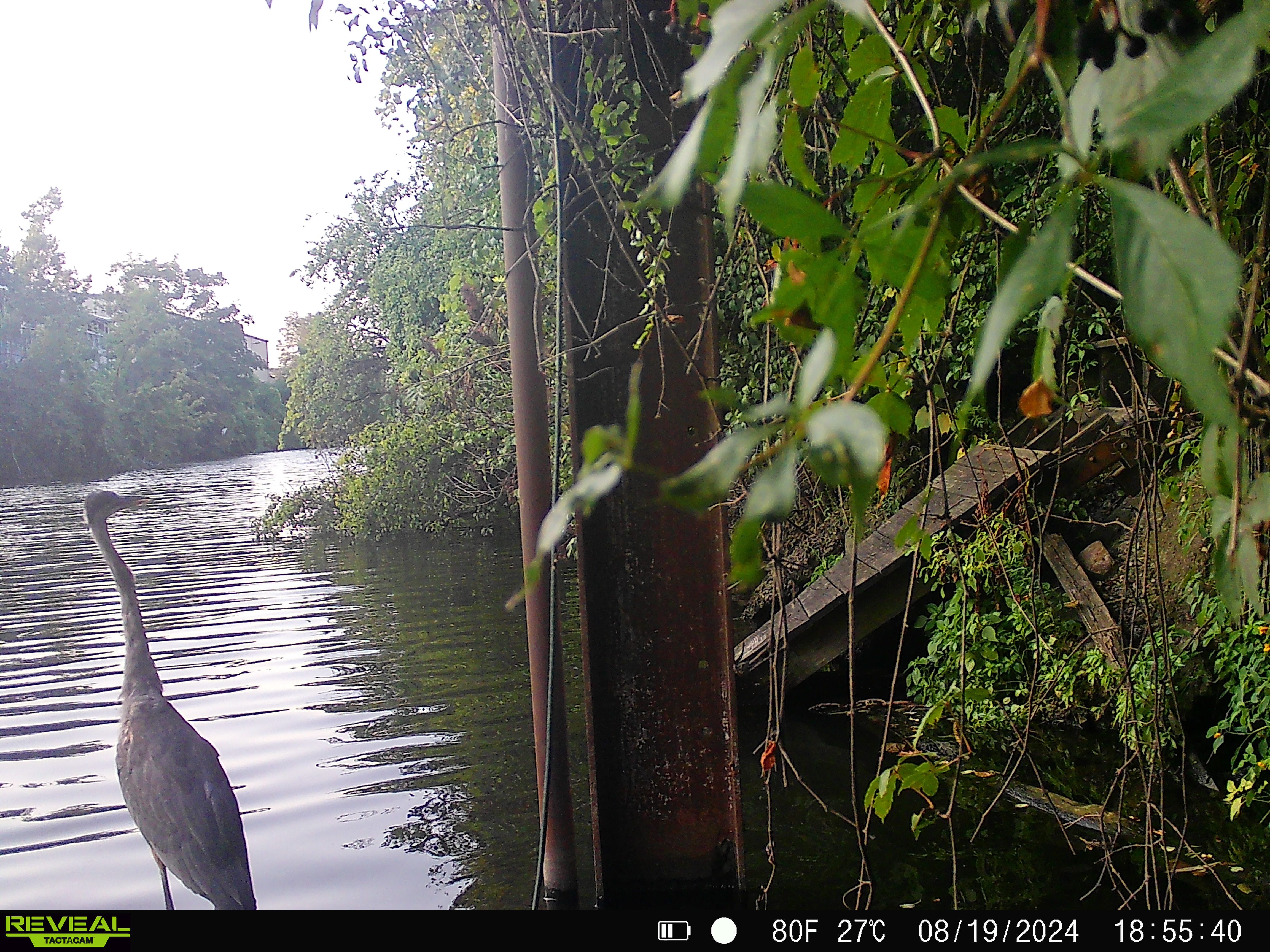
A good example of successfull Great Blue Heron classification
Project Workflow
- Process Images through the
SpeciesNetDeep Learning Computer Vision Model. - Associate inferences back to images via md5 hash - Data Cleaning.
- Explore Dataset - EDA.
- Plan for model fine-tuning & next steps.
Notebook for processing images on Kaggle:
The notebook took 10 hours to run - 7 hours of which was just spent on downloading and resizing images. This is why I used batching and multi-threading for the images, but yet it still takes a while to go through 100k s3 links. Surely there’s a better way.
Data Cleaning and EDA
Our primary goal with image classification - before releasing a model - is to confirm that predictions are “accurate enough”. This generally takes shape by having a holdout set of images with known (human graded) classes the ai doesn’t have access to. In our situation, we don’t have this quite yet - images are being labeled and classifications are on the production server - but the speciesnet ensemble doesn’t yet have a fine-tuning or base truth approach listed.
Ultimately this would let us “vote” on identifying species in photos using AI.
Since this is the first time we’re trying speciesnet, we’re going to do a few spot checks and EDA of the generated inference (predicted animals in photo) to understand how it performs.
Cleaning
After running the model we are left with a very long json file of 100k+ classifications and a pre-assembled [html pages][1] site through using megadetector-utils
Here’s an example of the structure for one image where a great blue heron was classified:
{
    "filepath": "images/batch_5/bada276600ce2790b1d2877e7d6e7a25.jpg",
    "classifications": {
    "classes": [
        "96fe1a07-7ef1-4a2f-99e1-ec2c9a78b532;aves;pelecaniformes;ardeidae;ardea;herodias;great blue heron",
        "bfa75aeb-3187-48fe-95b9-f171465cc984;aves;pelecaniformes;ardeidae;ardea;cocoi;cocoi heron",
        "b1352069-a39c-4a84-a949-60044271c0c1;aves;;;;;bird",
        "f8db21f0-6b79-4444-8be4-b87906d56e6a;aves;pelecaniformes;ardeidae;ardea;albus;great egret",
        "1110460b-7f99-405b-a9b0-65a09ecccca1;aves;pelecaniformes;ardeidae;tigrisoma;lineatum;rufescent tiger-heron"
    ],
    "scores": [
        0.7359567880630493,
        0.07253273576498032,
        0.04953608289361,
        0.03795544430613518,
        0.008134812116622925
    ]
    },
    "detections": [
    {
        "category": "1",
        "label": "animal",
        "conf": 0.8977401256561279,
        "bbox": [
        0.0,
        0.0,
        0.3460410535335541,
        0.9453125
        ]
    }
    ],
    "prediction": "96fe1a07-7ef1-4a2f-99e1-ec2c9a78b532;aves;pelecaniformes;ardeidae;ardea;herodias;great blue heron",
    "prediction_score": 0.7359567880630493,
    "prediction_source": "classifier",
    "model_version": "4.0.1a"
}
First, we need to extract data from the JSON file into a dataframe so we can more easily parse through some questions. Looking at the JSON structure, we need the filepath, a paired list of the classifications and their scores, and a paired list of any detections and their scores. Speciesnet does ultimately give us a prediction inference based on a taxonomic hierarchy decision set, but to learn more, we want the full dataset minus some very low confidence prections. My preference for this step is to stick to pure python for parsing - aiming to create a list of dicts for generating a dataframe. In my opinion, this is a lot easier to read than the jargon in the pandas library for extraction.
_CONF = 0.3 # Master Setting for confidence or score threshold

# Function for pairing classification and score
def get_high_score_classes(scores, classes, threshold=_CONF):
    return [{"score": f'{score:.2f}', "class": cls} for score, cls in zip(scores, classes) if score > threshold]

# Function for pairing detection and score
def get_high_conf_detections(detections, target_label, threshold=_CONF):
    return [(f'{det["conf"]:2f}', det["label"]) for det in detections if det["label"] == target_label and det["conf"] > threshold]

# Staged Configuration
master_data = []

# Open and loop over json file
with open(master_json, "r") as f:
    data = json.load(f)
    for image in data["predictions"]:
        high_score_classes = get_high_score_classes(
            image["classifications"]["scores"],
            image["classifications"]["classes"],
            _CONF
        )
        master_data.append({
            "imageName": image["filepath"].split("/")[2],
            "nDetections_animal": len(get_high_conf_detections(image["detections"], "animal", _CONF)),
            "nDetections_human": len(get_high_conf_detections(image["detections"], "human", _CONF)),
            "nDetections_vehicle": len(get_high_conf_detections(image["detections"], "vehicle", _CONF)),
            "nClassifications": len(high_score_classes),
            "highScoreClasses": high_score_classes

        })

# Previous work identified 55363 as our heron example index -
display(master_data[55363])
This script processes all 100k+ predictions in about 7 seconds, extracting a preferable starting point for EDA.
The heron example:
{'imageName': 'bada276600ce2790b1d2877e7d6e7a25.jpg',
 'nDetections_animal': 1,
 'nDetections_human': 0,
 'nDetections_vehicle': 0,
 'nClassifications': 1,
 'highScoreClasses': [{
    'score': '0.74',
    'class': '96fe1a07-7ef1-4a2f-99e1-ec2c9a78b532;aves;pelecaniformes;ardeidae;ardea;herodias;great blue heron'
 }]
}
From here it’s very simple to just define the dataframe as df = pd.DataFrame(master_data)
Next, we want to make sure that each row in our dataframe contains exactly one class prediction. This step is important because if an image has more than one classification above our threshold, while we’re ok with having more than one classification per image (sometimes there are more than 1 species in a photo!), we want to know the high score classification(s) in each photo.
For example:
imageName: '269ed4dcbaf7419a1d00e6957ff2beff.jpg'
highScoreClasses:
  [
    {'score': '0.57', 'class': 'f1856211-cfb7-4a5b-9158-c0f72fd09ee6;;;;;;blank'},
    {'score': '0.37', 'class': 'd372cda5-a8ca-4b7b-97ed-4e4fab9c9b4b;mammalia;cetartiodactyla;suidae;sus;scrofa;wild boar'}
  ]
With df2 = df.explode("highScoreClasses", ignore_index=True) turns into:
imageName: '269ed4dcbaf7419a1d00e6957ff2beff.jpg'
highScoreClasses:
  [
    {'score': '0.57', 'class': 'f1856211-cfb7-4a5b-9158-c0f72fd09ee6;;;;;;blank'}
  ]
imageName: '269ed4dcbaf7419a1d00e6957ff2beff.jpg'
highScoreClasses:
  [
    {'score': '0.37', 'class': 'd372cda5-a8ca-4b7b-97ed-4e4fab9c9b4b;mammalia;cetartiodactyla;suidae;sus;scrofa;wild boar'}
  ]
This increased our row count from 104937 to 107535
Now we’re going to parse that very long taxonomic string into the common name ‘most specific’ name that occupies the last item in the semicolon separated list. This is a very long line of code - but, chatGPT helped puzzle through it and we’re going to use it.
# Split by ';' and take the last part
df2['class'] = df2['highScoreClasses'].apply(lambda d: d.get('class') if isinstance(d, dict) else None).str.split(";").str[-1]
Last, we want to re-associate some of the data originally pulled for the predictions - namely the datetime and the publicURL for each image. To do that we will merge the predictions with the metadata - both files were downloaded as CSVs at this stage or early on in the process and can be linked via the unique mediaID (a simple parse of the imageName).
merged_df = pd.merge(metadata, predicts, on="mediaID", how="inner")
After running this the first time, the merged_df had a few hundred more rows than the predictions dataset - so, the metadata probably has duplicated media ids. This is pretty normal because the image uploading process doesn’t include deduplication. So, before the merge I added metadata_unique = metadata.drop_duplicates(subset=['mediaID'])
merged_df = pd.merge(metadata_unique, predicts, on="mediaID", how="inner")
Selecting our needed columns gives us:
Cleaned Data
| mediaID | timestamp | publicURL | folderName | animal | human | vehicle | class |
|---|---|---|---|---|---|---|---|
| 113f9bb5…39b0 | 2024-12-25 15:29:24 | https://urbanriverrangers…SYFW01868.jpg | 2025-01-04_UR027 | 0 | 1 | 0 | human |
| 871315ba…d6de | 2024-12-25 15:29:24 | https://urbanriverrangers…SYFW01869.jpg | 2025-01-04_UR027 | 0 | 1 | 0 | human |
| 991baede…a9db | 2024-12-25 15:29:24 | https://urbanriverrangers…SYFW01870.jpg | 2025-01-04_UR027 | 0 | 1 | 0 | human |
| 32c8912b…f68c | 2024-12-25 15:29:26 | https://urbanriverrangers…SYFW01871.jpg | 2025-01-04_UR027 | 0 | 0 | 0 | blank |
| f4ba4a3d…8d0a | 2024-12-25 15:29:26 | https://urbanriverrangers…SYFW01872.jpg | 2025-01-04_UR027 | 0 | 0 | 0 | blank |
Exploratory Analysis
First let’s just get a list of the top 20 classifications and graph it - there is an overwhelming number of blanks - so we’re going to use a log-scale.
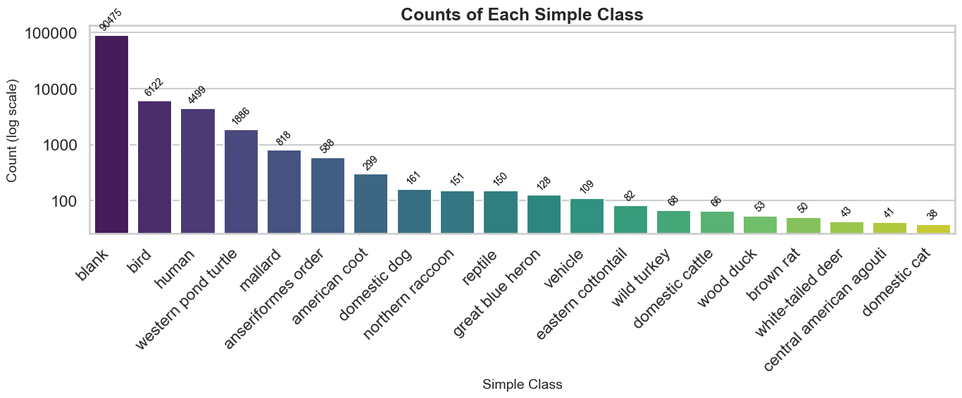 ..and by the numbers:
| # | Class | Count | % |
|---|---|---|---|
| 1 | blank | 90475 | 84.1 |
| 2 | bird | 6122 | 5.7 |
| 3 | human | 4499 | 4.2 |
| 4 | western pond turtle | 1886 | 1.8 |
| 5 | mallard | 818 | 0.76 |
| 6 | anseriformes order | 588 | 0.55 |
| 7 | american coot | 299 | 0.28 |
| 8 | domestic dog | 161 | 0.15 |
| 9 | northern raccoon | 151 | 0.14 |
| 10 | reptile | 150 | 0.14 |
| 11 | great blue heron | 128 | 0.12 |
| 12 | vehicle | 109 | 0.10 |
| 13 | eastern cottontail | 82 | 0.076 |
| 14 | wild turkey | 68 | 0.063 |
| 15 | domestic cattle | 66 | 0.061 |
| 16 | wood duck | 53 | 0.049 |
| 17 | brown rat | 50 | 0.046 |
| 18 | white-tailed deer | 43 | 0.040 |
| 19 | central american agouti | 41 | 0.038 |
| 20 | domestic cat | 38 | 0.035 |
An overwhelming 84% of the images are blanks according to speciesnet. Given probably more than a few of these are just false negatives, but still - it mirror’s what we’ve been experiencing in labeling activities: a whole lot of boring.
For completeness - let’s also look at the least frequent 20. Most of these are ties because they are n=1:
| # | Class | Count | % |
|---|---|---|---|
| 65 | rattus species | 1 | 0.001 |
| 66 | greater roadrunner | 1 | 0.001 |
| 67 | scaly ground-roller | 1 | 0.001 |
| 68 | merle dyal malgache | 1 | 0.001 |
| 69 | red acouchi | 1 | 0.001 |
| 70 | blood pheasant | 1 | 0.001 |
| 71 | white-lipped peccary | 1 | 0.001 |
| 72 | red fox | 1 | 0.001 |
| 73 | desert cottontail | 1 | 0.001 |
| 74 | rufescent tiger-heron | 1 | 0.001 |
| 75 | common wombat | 1 | 0.001 |
| 76 | african elephant | 1 | 0.001 |
| 77 | bearded pig | 1 | 0.001 |
| 78 | eastern chipmunk | 1 | 0.001 |
| 79 | fossa | 1 | 0.001 |
| 80 | l’hoest’s monkey | 1 | 0.001 |
| 81 | house rat | 1 | 0.001 |
| 82 | bobcat | 1 | 0.001 |
| 83 | nine-banded armadillo | 1 | 0.001 |
| 84 | guenther’s dik-dik | 1 | 0.001 |
There are clearly some errors in classification. This run of the model was run without any geofencing to avoid collapsing low classification confidences into a higher “animal” taxonomy level. Probably a large portion of these would not exist. Increasing our _CONF threshold to >0.80 reduced our species counts to 27 for example instead of 84. Unfortunately playing with this value drops some true detections in favor of having none at all - we will explore this type of decision more after we have an opportunity for fine-tuning.
Another popular angle in conservation is looking for patterns in usage by time of day. Here’s a chart for the top 10 classes and all of our pictures.
This could be further subsetted into seasons but for this first pass we are just getting an understanding.
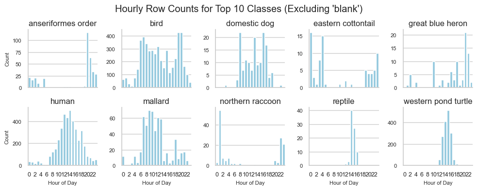
There are definiely nocturnal patterns already emerging in a “we aren’t totally confident it got it right all that often” dataset.
For example, we see humans follow a normal bell curve pattern of visitation, dogs seem to spike in the morning, noon, and evening (for walkies I hope), and species like cottontails and raccoons show up when the lights go out and nobody is around.
Same plot but with a shared y-axis:
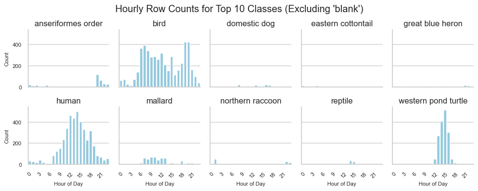
Here we get a sense of who we’re sharing the wild mile with: birds and turtles (not western pond turtles, but we’ll fix that soon)
The full cleaning and eda notebook is embedded in all of its’ chaotic glory here:
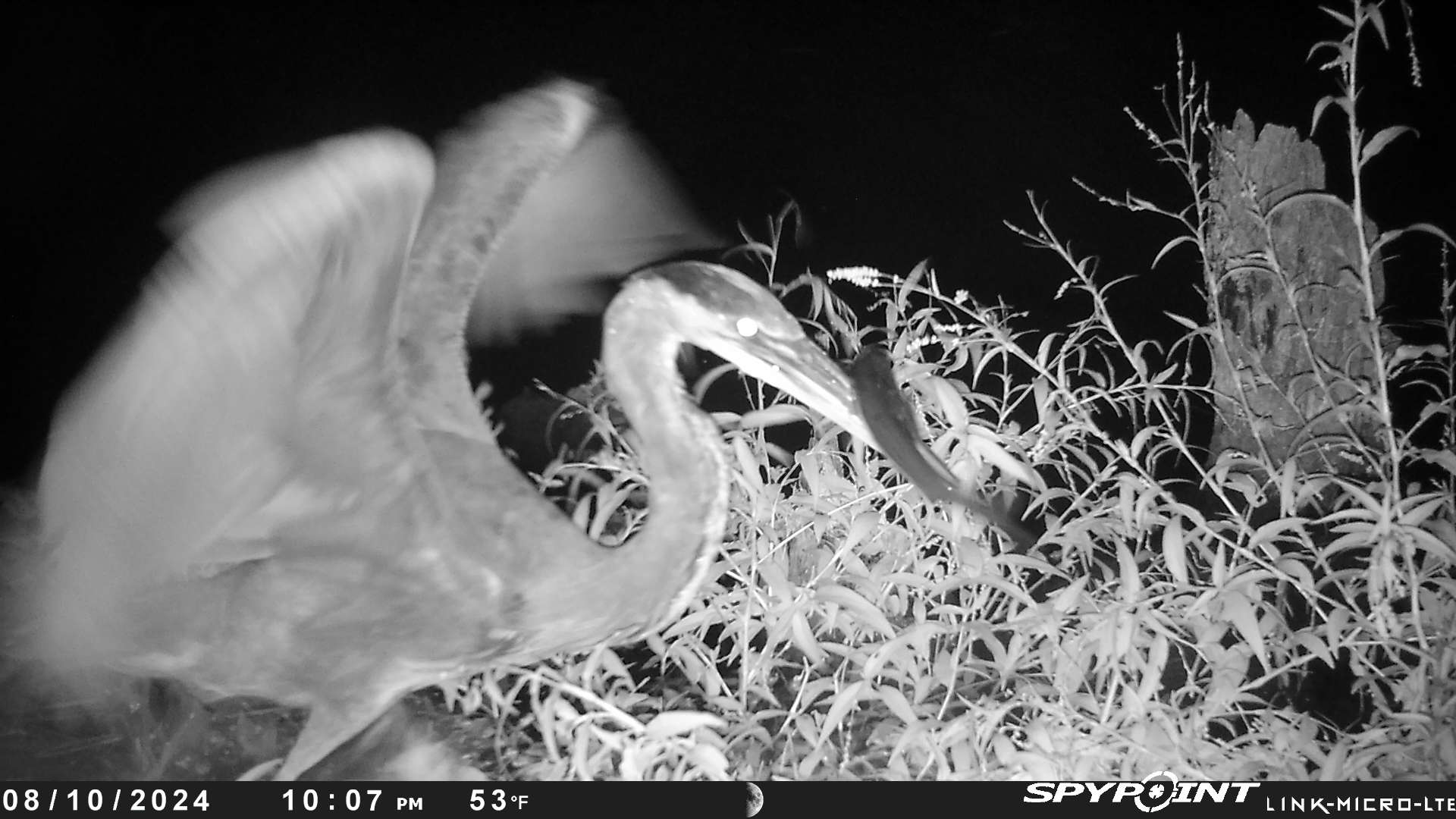
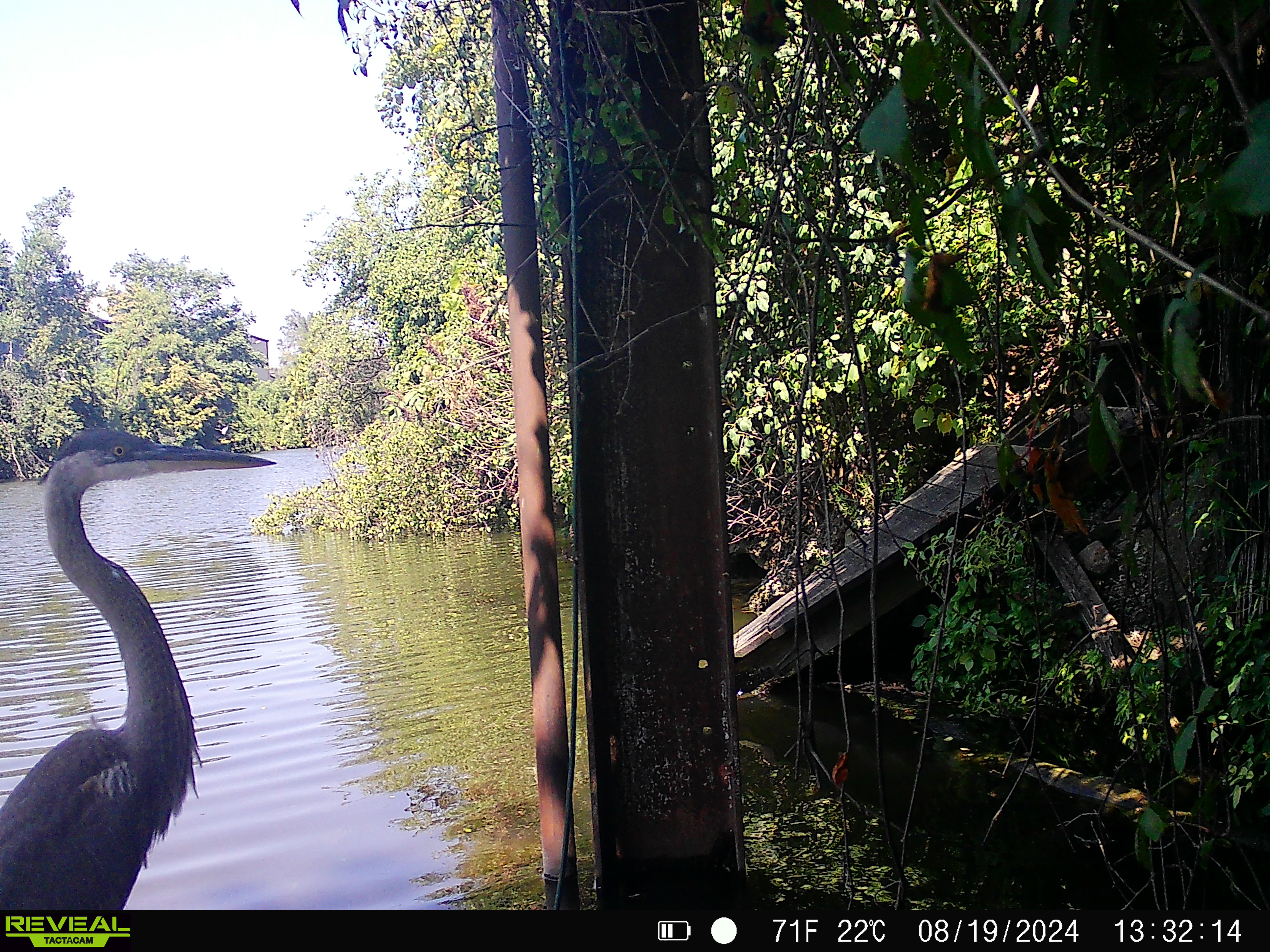
Obligatory example of good classification
Next Steps
Overall, we succeeded in using the SpeciesNet ensemble released by google. We were able to generate over 100k predictions for our camera trap images, and parse those predictions into a useable structure for analysis and validation.
The first attempts at this used a gps geofence parameter and full resolution images. We seemed to have better luck by resizing the images before inference - something that speciesnet does also do - but perhaps the two stage downsampling of the images led to a more familiar (lower resolution) image like those used for training initially.
The next step I’m excited about involve learning how to deploy this model to huggingface through gradio & then, after getting human graded image ids, working on fine tuning SpeciesNet to our image types.
The goal here is to reduce the boring parts of image labeling - something MegaDetector and SpeciesNet did excellently.
To get started on parsing the false positive (species who don’t belong) I build a webapp to interact with gbif data.
This is something you can both use here.
And read about here.
SpeciesNet was described by Gadot et al.1
-
Gadot, T., Istrate, Ș., Kim, H., Morris, D., Beery, S., Birch, T., & Ahumada, J. (2024). To crop or not to crop: Comparing whole-image and cropped classification on a large dataset of camera trap images. IET Computer Vision. Wiley Online Library. ↩